Project: High Angular Resolution Diffusion Imaging Tools
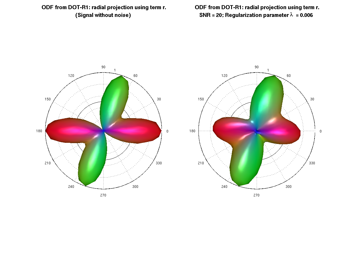
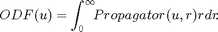
Example to illustrate the Revisited version of the Diffusion Orientation Transform (DOT) method using real spherical harmonic basis. The ODF is the radial projection of the propagator computed by the following expression:
- Language: MATLAB(R)
- Author: Erick Canales-Rodríguez, Lester Melie-García, Yasser Iturria-Medina, Yasser Alemán-Gómez
- Date: 2013, Version: 1.2
Contents
- Parameters for reconstruction: All this part is equal for each voxel
clear all; close all; clc;

% - Loading the measurement scheme

grad = load('/sampling_and_reconstruction_schemes/On_the_sphere/70_shell.txt');
% grad is a Nx3 matrix where grad(i,:) = [xi yi zi] and sqrt(xi^2 + yi^2 + zi^2) == 1 (unit vectors).
display(['The measurement scheme contains ' num2str(size(grad,1)) ' directions']);

% - Loading the reconstruction scheme (mesh where the ODF will be reconstructed)
%   ---------------------------------
% unit vectors on the sphere
disp(' ')
V = load('/sampling_and_reconstruction_schemes/On_the_sphere/724_shell.txt');
% facets
display(['The reconstruction scheme contains ' num2str(size(V,1)) ' directions']);
F = load('/sampling_and_reconstruction_schemes/On_the_sphere/724_sphere_facets.txt');
disp(' ');

%  --- Regularization parameter
Lambda = 0.006;
display(['The regularization parameter Lambda is ' num2str(Lambda) ',']);
display ('like in the Descoteaux paper "Regularized, Fast, and Robust Analytical Q-Ball Imaging".');

% --- real spherical harmonic reconstruction: parameters definition --- %
[Lmax Nmin] = obtain_Lmax(grad);
if Lmax >= 8
    Lmax = 8;
end
display(['The maximum order of the spherical harmonics decomposition is Lmax = ' num2str(Lmax) '.']);

[basisG, thetaG, phiG] = construct_SH_basis (Lmax, grad, 2, 'real');
[basisV, thetaV, phiV] = construct_SH_basis (Lmax, V, 2, 'real');
K = []; Laplac2 = [];
for L=0:2:Lmax
    for m=-L:L
        factor_dot1 = ((-1)^(L/2))*gamma(1+ L/2)./gamma((1 + L)/2);
        K = [K; factor_dot1];
        Laplac2 = [Laplac2; (L^2)*(L + 1)^2];
    end
end
Laplac = diag(Laplac2);

% Creating the kernel for the reconstruction
A = recon_matrix(basisG,Laplac,Lambda);
% where A = inv(Ymatrix'*Ymatrix + Lambda*Laplacian)*Ymatrix';
% and Ymatrix = basisG.
% The matrix, A, is the same for all the voxels

A0 = recon_matrix(basisG,Laplac,0);
% Note that in this case we created an additional matrix A0,
% this matrix is different to A because the regularization parameter is set
% to zero (Lambda = 0).
The measurement scheme contains 70 directions

The reconstruction scheme contains 724 directions

The regularization parameter Lambda is 0.006,
like in the Descoteaux paper "Regularized, Fast, and Robust Analytical Q-Ball Imaging".
The maximum order of the spherical harmonics decomposition is Lmax = 8.
- Simulated diffusion MRI signal using a multi-tensor model
% --- Experimental parameters --- %
% b-value
b = 4*10^3;% s/mm^2
% diffusivities
lambda1 = 1.5*10^-3;% mm^2/s
lambda2 = 0.3*10^-3;% mm^2/s
% S0 is the image at b-value = 0
S0 = 100;
% Signal to noise ratio
SNR = 20;
display(['The signal to noise ratio in this experiment is SNR = ' num2str(SNR) '.']);
% Add a measurement with b-value = 0 into the gradient matrix (standard format in which the signal is measured in the scanner)
grad = [0 0 0; grad];

% --- Intravoxel properties --- %
% Using a mixture of two fibers (more fibers can be used)
% volume fraction for each fiber (the sum of this elemenst is 1 by definition)
f1 = 0.5; f2 = 0.5;
% angular orientation corresponding to each fiber (main eigenvector for each diffusion tensor)
anglesF = [0  0;
           70 0];
% [ang1 ang2]: -> ang1 is the rotation in degrees from x to y axis (rotation using the z-axis);
%                 ang2 is the rotation in degrees from the x-y plane to the z axis (rotation using the y axis)
% anglesF(i,:) defines the orientation of the fiber with volume fraction fi.

%  --- Computation of the diffusion signal using the above experimental parameters and intravoxel properties %
% *** Signal with realistic rician noise
add_rician_noise = 1;
S = create_signal_multi_tensor(anglesF, [f1  f2],...
    [lambda1, lambda2, lambda2], b, grad, S0, SNR, add_rician_noise);

% *** Ideal signal (no noise)
add_rician_noise = 0;
Snonoise = create_signal_multi_tensor(anglesF, [f1  f2],...
    [lambda1, lambda2, lambda2], b, grad, S0, SNR, add_rician_noise);
The signal to noise ratio in this experiment is SNR = 20.
- Isolate the S0 component from the signal
% --- find zeros
grad_sum = sum(abs(grad),2);
ind_0 = find( grad_sum == 0);
S0_est = max(S(ind_0));
S(ind_0) = []; Snonoise(ind_0) = [];
grad(ind_0,:) = [];
- ODF from the signal without noise
ADCnonoise = abs(-log(Snonoise/S0)/b)';
NewSignal_nonoise = ADCnonoise(:).^(-1/2);

coeff0 = A0*NewSignal_nonoise;
ss0 = coeff0.*K;
ODFnnoise = basisV*ss0;
ODFnnoise = ODFnnoise - min(ODFnnoise);
ODFnnoise = ODFnnoise/sum(ODFnnoise); % normalization
- Regularized ODF from the noised signal
display('This is the real/effective time required for computing the ODF at each voxel:')
tic
ADC = abs(-log(S/S0_est)/b)';

% --- ADC denoising
ADCd = (basisG*(A*ADC(:))); % denoised using the spherical harmonic series
NewSignal = ADCd(:).^(-1/2);

%coeff = A0*NewSignal;
coeff = A*NewSignal;
ss = coeff.*K;
ODF = basisV*ss;
ODF = ODF - min(ODF);
ODF = ODF/sum(ODF); % normalization
toc
This is the real/effective time required for computing the ODF at each voxel:
Elapsed time is 0.000369 seconds.
- Plots
% --- opengl('software');
feature('UseMesaSoftwareOpenGL',1);

set(gcf, 'color', 'white');
screen_size = get(0, 'ScreenSize');
f1 = figure(1); hold on;
set(f1, 'Position', [0 0 screen_size(3) screen_size(4) ] );
cameramenu;
% -----
Origen = [0 0 0.25]; % Voxel coordinates [x y z] where the ODF will be displayed
angle = 0:.01:2*pi;
R = ones(1,length(angle));
R1 = R.*f2/f1;
subplot(1,2,1)
polarm(angle,R,'k'); hold on; polarm(angle, R1,'k');
% the ODF is scaled only for the display
plot_ODF(ODFnnoise./max(ODFnnoise), V, F, Origen);
title({'\fontsize{14} ODF from DOT-R1: radial projection using term r.';'(Signal without noise)'},'FontWeight','bold');
axis equal; axis off;

subplot(1,2,2)
polarm(angle,R,'k'); hold on; polarm(angle, R1,'k');
% the ODF is scaled only for the display
plot_ODF(ODF./max(ODF),V, F, Origen);

title({'\fontsize{14} ODF from DOT-R1: radial projection using term r.';...
       ['SNR = ' num2str(SNR) '; Regularization parameter {\lambda}  = ' num2str(Lambda)]},'FontWeight','bold');
axis equal; axis off;